Lab 5: Linear PID control and Linear interpolation

Bluetooth Communication and PID Code

Data communication to and from the computer and Artemis were handeled similar to previous labs. The PID.CONTROL command is used to send the start flag and the Kp, Ki, Kd, and target distance: ble.send_command(CMD.PID_CONTROL, ".05|0|6|300") # P|I|D. The Arduino recieves the gains:

    case PID_CONTROL: {
    pid_start = 1;
    // Get PID parameters over BLE
    success = robot_cmd.get_next_value(Kp);
    if (!success) return;
    success = robot_cmd.get_next_value(Ki);
    if (!success) return;
    success = robot_cmd.get_next_value(Kd);
    if (!success) return;
    success = robot_cmd.get_next_value(target_tof);
    if (!success) return;
    tx_estring_value.clear();
    }

The main loop is responsible for running the runPID() function which collects the ToF data and internally runs the pid_speed_ToF() responsible for calculating the speed based on PID control feedback. The calculated speed is then passed into the forward() and reverse() functions from Lab 4. The function is run until the PID data array is filled (500 in this case).

void runPID(){
  start_time_pid = millis();

  for (int i = 0; i < pid_len; i++) {
    distanceSensor1.startRanging();
    pid_time[i] = millis() - start_time_pid;

    pid_tof[i] = distanceSensor1.getDistance();

    distanceSensor1.clearInterrupt();
    distanceSensor1.stopRanging();

    pid_speed[i] = pid_speed_ToF(Kp, Ki, Kd, pid_tof[i], target_tof);
    pid_p[i] = Kp * pos_error;
    pid_i[i] = Ki * integral_error;
    pid_d[i] = Kd * d_term;
  }
  stop();
  pid_start = 0;
  sendPIDData();     
}

Below is the int pid_speed_ToF() function. Note that after calculating the PID speed is calculated, there are various IF statments to account for the motor deadband, direction, stopping tolerance, and max speed. Effectively, the function logic flows as follows:

1. Calculate PID Speed from gains and error
2. If the speed is <1 it means we are effectively at our target and can stop
3. If we are not yet close enough to the target we check to ensure our set speed is lower than the max speed (in either direction). If it isn’t we bring the speed down to maxSpeed
4. If the speed falls within our deadband range from Lab 4 (PWM of 35), the PWM signal is brought up to 35
5. The set speed is passed into the reverse() or forward() function based on its sign

int pid_speed_ToF(float Kp, float Ki, float Kd, float pos_cur, float pos_targ){
  
  // Varaible Init
  time_cur = millis();
  dt = time_cur-time_prev;
  time_prev = time_cur;
  pos_error = pos_cur-pos_targ; // Position error
  d_term = (pos_error-prev_error)/dt; // Derivative term
  integral_error = integral_error + (pos_error*dt); // Integral Term

  // Set Speed PID Calculation
  int speed_set = ((Kp*pos_error) + (Ki*pos_error*dt) + (Kd*d_term)); // PID speed control

  // Set tolerance
  if (abs(speed_set) < 1){
    stop();
  }
  // If saturated (pos dir), set speed to max speed 
  if (speed_set > maxSpeed){
    speed_set = maxSpeed;
  }
  // If saturated (neg dir), set speed to max speed 
  if (speed_set < (-1*maxSpeed)) {
      speed_set = -1*maxSpeed;
  }
  // Set min speed to min PWM value from Lab 4
  if ((speed_set < minSpeed) && (speed_set > 0)) {
      speed_set = minSpeed;
  }
  // Set min speed to min PWM value from Lab 4
  if ((speed_set > (-1*minSpeed)) && (speed_set < 0)) {
      speed_set = -1*minSpeed;
  }
  // Set forward speed
  if (speed_set > 0){
    forward(speed_set);
  }
    // Set backwards speed
  if (speed_set < 0){
    reverse(-1*speed_set);
  }

prev_error = pos_error;
return speed_set;

}

After the data is collected, it is sent back to the computer over Bluetooth via the sendPIDData() function. On my computer the data is piped into a CSV file via my notification handler. From there, the data is plotted for visualization.

PID Control and Tuning

Range/Sampling Time Discussion

The following code was implemented to ensure that new ToF values were returned at least every 35ms. This is vital in PID control as we want to make sure we are re-calculating our speed frequently as possible even if it means trading off some accuracy. If new values are not recieved fast enough, the robot risks running into the wall or not being able to react fast enough to sudden changes in surroundings.

distanceSensor2.setDistanceModeLong();
distanceSensor2.setTimingBudgetInMs(35);
distanceSensor2.setIntermeasurementPeriod(40);

Proportional Control

For this lab the car starts roughly 2m-4m from the wall and is intended to stop 300mm from the wall. As a result, ToF readings (in mm) start at 2000-4000. For this lab, the intention is to keep the car speed to no more than ~150. If we focus on the very start of running the car, the error is roughly 3000-300 = 2700. Thus, my propotional gain values (which get multiplied by the 2700mm error) were in the range of .05 - .08 throughout tuning to keep us in the 100-150 PWM when at these large distances from the wall at the start. When the error gets very small, the Kp term is not large enough to provide the minimum PWM to move the car. As a result, the deadband minimum speed was implemented.

Below are two videos of only proportional control implementation with the car starting at ~2500mm from the wall. The first is with Kp = 0.5 and the second with Kp = 0.8. You can see that with the increased proportional gain, the car was unable to stop which is why a Kd term is added in the next section:

PD Control

While soley propotional control proved to be fairly accurate (effectively stopping <4mm from the target), overshoot and ramming into the walls was still an issue at higher speeds. Thus, since I wanted to try increasing my speed I have to implement a derivative term. The derivative term helps to slow the car down proportional to the slope of the error. As the car approaches the wall the error is decreasing resulting in a negative derivative term that helps reduce the overall speed. You can see that with the same Kp = .08 value that previously crashed the car we are now able to stop early enough to avoid crashing with the addition of a derivative gain.

I ran the robot with the following gains Kp = .08 & Kd = 6

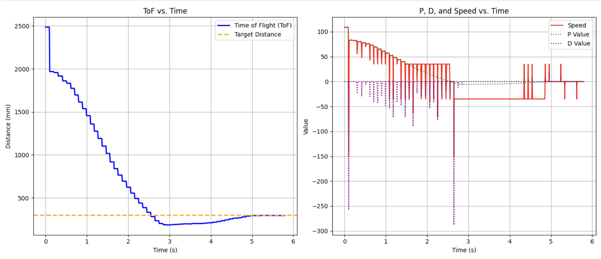
Discrete Kd values can be seen as the ToF values are unfotunely slow. When there is not a new ToF reading, the derivative term is zero as the current and previous error terms are the same until a new ToF reading comes in. To address this issue we extrapolate. Effectively, the derivative term is only slowing the car down at discrete intervals which is not enough to slow the car down in time at much higher speeds.

Extrapolation

Loop Speed Discussion (no Extrapolation)

My ToF returns new data every 108.21 ms on average which corresponds to a rate of 9.24 Hz. This large delay leads to the derivative issue mentioned above. When the code is sped up to eleminate waiting for a new ToF reading, the speed of the loop is now 172.27 Hz.

Extrapolation Implementation

The following extrapolation code was added to the runPID() function. Essentially, two distance arrays are used: tof_time[i] for ToF readings as they are ready and interpolated[counter] which stores interpolated data. Two time arrays are also implemented: tof_time[i] to store time intervals that the sensors collect data at (important for calculating slope) and times[counter] for constant running time (also used by the interpolator).

start_time_pid = millis()/1000;

for (int counter = 0; counter < pid_len; counter++) {

  times[counter] = millis()/1000 - start_time_pid;

  if (distanceSensor1.checkForDataReady()){
  tof_time[i] = millis();
  pid_tof[i] = distanceSensor1.getDistance();
  interpolated[counter] = pid_tof[i];
    
    if (i >= 1) {
      slope_ToF = (pid_tof[i] - pid_tof[i-1]) / (tof_time[i] - tof_time[i-1]);
    }
    curDistance = pid_tof[i];
    i++;

  }  
  else {
    if (i >= 1){
      curDistance = interpolated[counter-1] + (slope_ToF * (millis()/1000 - times[counter-1]));
      interpolated[counter] = curDistance;

    }
    else{
      interpolated[counter] = pid_tof[i];

    }
  }

Proportional Control with Extrapolation

I started with testing extrapolation with proportional control. After many many hours of debugging it finally worked (yielding the above extrapolation code)!

Here is a run with Kp set to 0.1

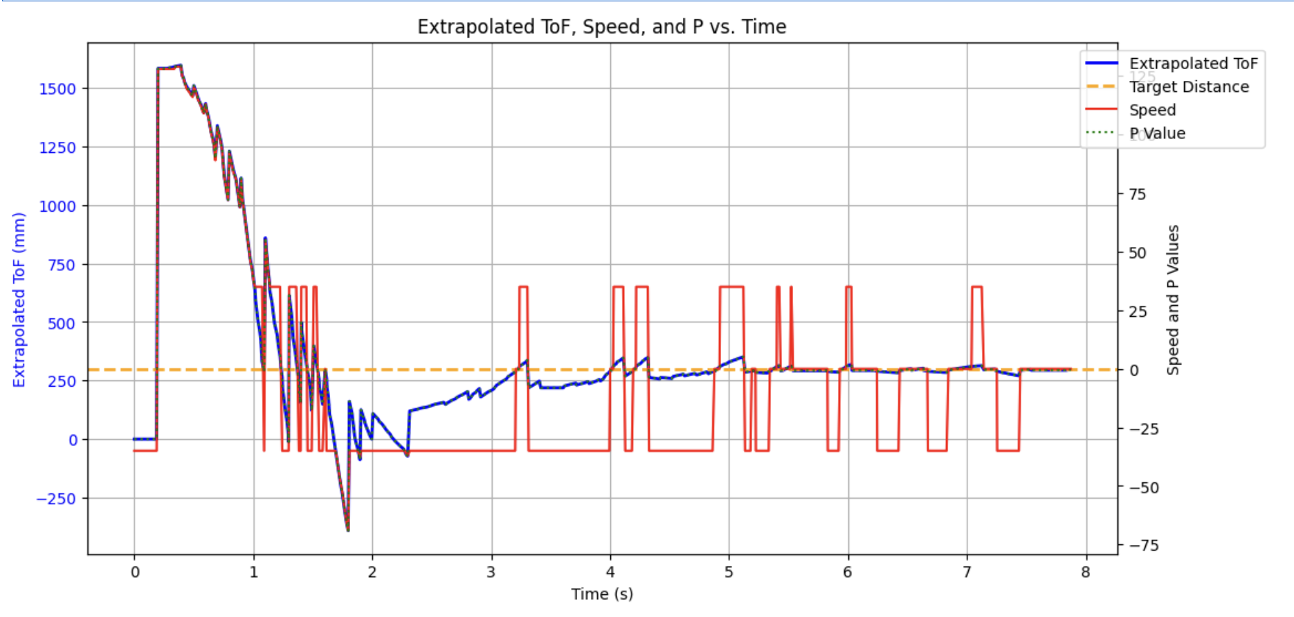
While the robot does eventually finish at the 1 ft target, it initially overshoots and has to backtrack. This is solved via implementing derivative control to help slow the robot down as the error decreases. When graphing the extrapolated data it follows the expected curve however would benefit from some low pass filtering in the future.

PD Control with Extrapolation

Here is the first test after addings the derivative term with extrapolation (PD control). Kp set to 0.1 and Kd set to 3

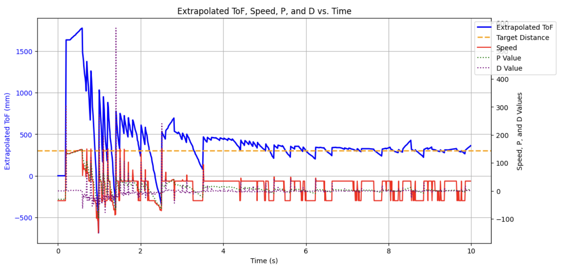
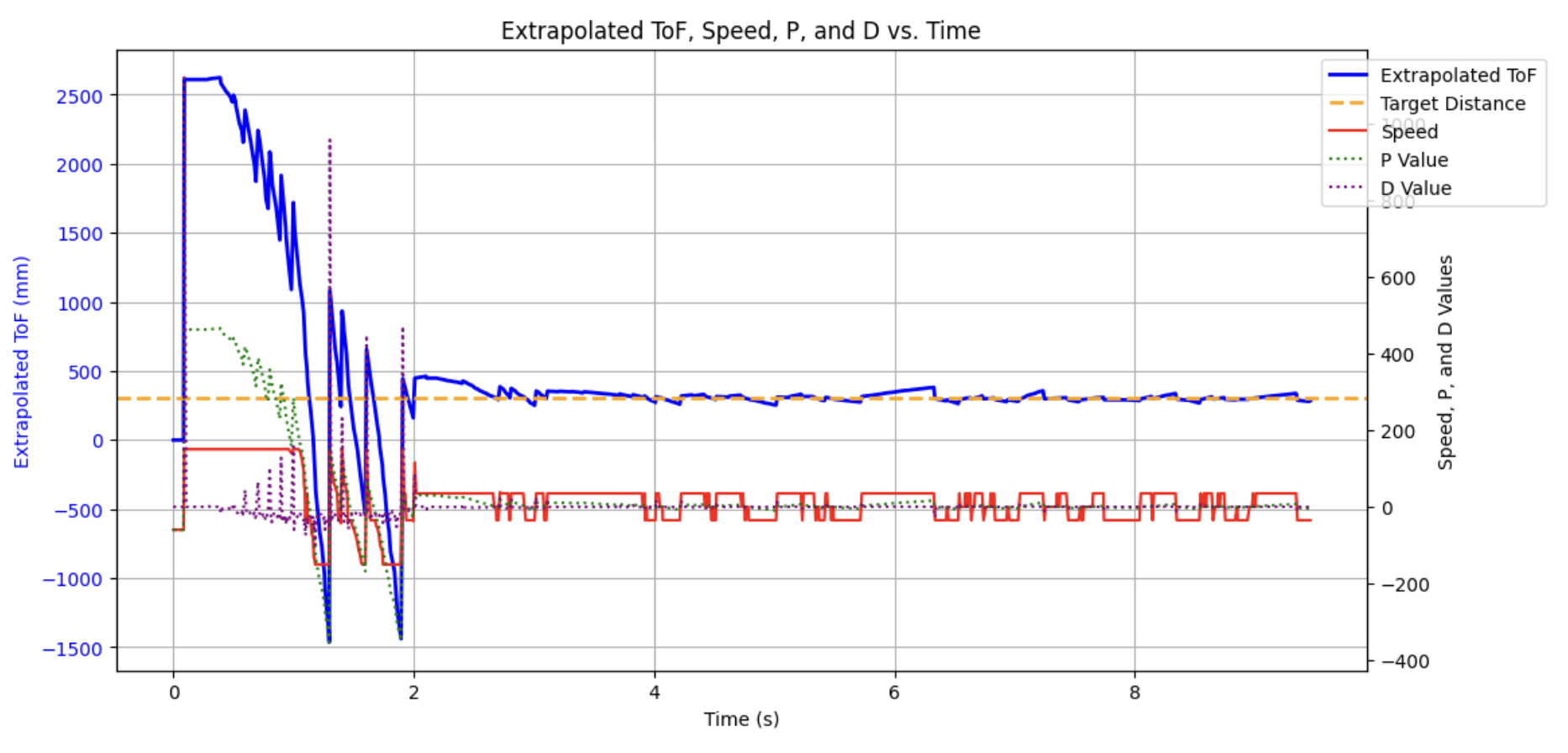
While the robot does reach the final 1ft target, it slows down a little earlier than it should. To account for this, the Kp term was increased to 0.2. For this final test I also tested to see how far I could back up the car and still have it reach the target distance. Here is the final video with Kp = 0.2 and the car started roughly 2.7m from the wall.

In conclusion, when comparing the extrapolated and non-extrapolated results, we can see the car far more able to slow down accurately. This allows for a overall faster speed without overshooting the target and crashing. With near zero steady state error, I did not find it necessary to implement integral control at the moment. However, the infastructure is in the code; if I wanted to use it I would just have to pass through an integral gain and tune!

Collaboration

I collaborated extensively on this project with Jack Long and Trevor Dales. I referenced Wenyi’s site for PID implementation code and Daria’s site for help with extrapolation. ChatGPT was used to help plot graphs.